# slit function
    # Define the slit function, slite_type can be 'rectangular', 'circular', or 'double'
def slit_function(slit_type,x,y,D,S,Height):
    if slit_type == 'rectangular':
        return rectangular_slit(x, y, D, Height)
    elif slit_type == 'circular':
        return circular_slit(x, y, D)
    elif slit_type == 'double':
        return double_slit(x, y, D, S,Height)
    else:
        raise ValueError("Invalid slit type. Choose 'rectangular', 'circular', or 'double'.")
# Define the slit patterns
def rectangular_slit(x, y, D, Height):
    # Create a rectangular slit pattern
    # The slit is centered at (0, 0) and has width D and height Height
    return (np.abs(x) < D/2) * (np.abs(y) < Height/2)
def circular_slit(x, y, D):
    # Create a circular slit pattern
    # The slit is centered at (0, 0) and has diameter D
    # The circular slit is defined by the equation x^2 + y^2 < (D/2)^2
    return (np.abs(x)**2+np.abs(y)**2)<(D/2)**2
def double_slit(x, y, D, S,Height):
    # Create a double slit pattern
    # The slits are centered at (-S/2, 0) and (S/2, 0) with width D and height Height
    slit1 = rectangular_slit(x + S/2, y, D, Height)
    slit2 = rectangular_slit(x - S/2, y, D, Height)
return slit1 + slit2Fourier Optics
- Input waveform or the aperture function is \(f(x,y)\).
- If \(f(x,y)\) is a plane monochromatic wave, then at z=0, the function can be written as \[ f(x,y)=A\exp[-j{2}\pi(\nu_{x}x+\nu_{y}y)] \]
- Where, A is the amplitude of the wave.
- \(\nu_x\) and \(\nu_y\) are spatial frequencies. \(v_{x}=\frac{k_{x}}{2\pi}\),\(\nu_{y}=\frac{k_{y}}{2\pi}\), \(k_{x}\) and \(k_y\) are spatial angular frequencies.
- \(k_x\), \(k_y\) and \(k_z\) are components of wave vector \(k\), \(k=\frac{2\pi}{\lambda}\), where \(\lambda\) is the wavelength of light.
- After traveling for distance d along the z axis, the wave will become, \(g(x,y)=Ae^{-jkd}\)
- More generally \(f(x,y)\) is a superposition integral of harmonic functions \[ f(x,y)=\iint_{-\infty}^{\infty} F_{1}(\nu_{x},\nu_{y})\exp[-j_{2}\pi(\nu_{x}x+\nu_{y})] \, d\nu_{x} \, d\nu_{y} \]
- \(F(\nu_{x},\nu_{y})\) is a complex envelope.
- Looking at the formula, it can be deduced that \(f(x,y)\) and \(F(\nu_{x},\nu_{y})\) are Fourier transform of one another.
- We can write, \(F(\nu_{x},\nu_{y})=\text{FT}[f(x,y)]\) and \(f(x,y)=\text{IFT}[F_{1}(\nu_{x},\nu_{y})]\)
- FT: Fourier transform, IFT: Inverse Fourier transform
- The harmonic function \(F(\nu_{x},\nu_{y})\) can be found from the input waveform by Fourier transform.
Transfer function of free space.
\[ H(\nu_{x},\nu_{v})=\exp\left(-j2\pi d\sqrt{ \lambda^{-2}-\nu_{x}^{2}-\nu_{y}^{2}}\right) \] - The output harmonic function at the image plan is \(F_2(\nu_{x},\nu_{y})\) - It can be found as \[ F_2(\nu_{x},\nu_{y})=H(\nu_{x},\nu_{y})F_1(\nu_{x},\nu_{y}) \] - From that the waveform \(g(x,y)\) at the output plane can be found as, \[ g(x,y)=\text{FT}[F_{2}(\nu_{x},\nu_{y})] \]
Fresnel approximation
- Under Fresnel approximation, the expression for the transfer function reduces to \[ H(\nu_{x},\nu_{v})\approx H_{o}\exp\left[j_{2}\pi d(\nu_{x}^{2}+\nu_{y}^{2})\right] \]
- Where, \(H_o=e^{-jkd}\)
- Condition for validity of Fresnel approximation is that the Fresnel number \(N_F\ll_{}1\), where \(N_F=\frac{a^{2}}{\lambda d}\), d is the largest radial distance at the output plane.
Fraunhofer approximation
- Additional condition for Fraunhofer approximation, in addition to the conditions in Fresnel approximation is \(N_F'\ll_{}1\), where, \(N_F=\frac{b^{2}}{\lambda d}\), where b is the slit size.
- Under Fraunhofer approximation the waveform \(g(x,y)\) at the output plane is \[ g(x,y)\approx h_{o}\text{F}\left(\frac{x}{\lambda d},\frac{y}{\lambda d} \right) \]
- Where F is the Fourier transform of input waveform \(f(x,y)\), evaluated at \(\nu_{x}=\frac{x}{\lambda d}\) and \(\nu_{y}=\frac{y}{\lambda d}\).
- Where \(h_{o}=\frac{j}{\lambda d}e^{-jkd}\)
# Transfer function
def transfer_function(method,slit_type,z,wavelength,D,S,Height):

    wavelength=wavelength*1e-6  # Convert wavelength to mm
    k=2*np.pi/wavelength  # Wave number in radians/mm
    x=np.linspace(-2,2,3200)  # x-axis range in milimeters
    y=np.linspace(-2,2,3200)  # y-axis range in milimeters
    xv,yv=np.meshgrid(x,y)    # Create a meshgrid for x and y
    f= slit_function(slit_type, xv, yv,D,S,Height)  # Generate the slit function based on the specified type
    F=fft2(f)  # Fourier transform of the slit function
    kx=fftfreq(len(x),np.diff(x)[0])*2*np.pi    # Spatial angular frequency in radians/mm
    ky=fftfreq(len(y),np.diff(y)[0])*2*np.pi    # Spatial angular frequency in radians/mm
    kxv, kyv = np.meshgrid(kx, ky)            # Create a meshgrid for kx and ky
    nux=kxv/(2*np.pi)                       # Spatial frequency in radians/mm, different from angular frequency
    nuy=kyv/(2*np.pi)                       # Spatial frequency in radians/mm
    # Calculate the transfer function based on the method
    if method == 'exact':
        g=ifft2(F*np.exp(-1j*z*np.sqrt(k**2-kxv**2-kyv**2)))
        return x,y,f,g
    if method == 'Fresnel':
        H0=np.exp(-1j*k*z)
        g=ifft2(F*H0*np.exp(1j*(np.pi)*wavelength*z*(nux**2+nuy**2)))
        return x,y,f,g
    if method == 'Fraunhofer':
        h0=(1j/(wavelength*z))*np.exp(-1j*k*z)
        g=fftshift(F)*h0
        x=fftshift(kxv)*(wavelength*z)
        y=fftshift(kyv)*(wavelength*z)
        return x,y,f,g
    else:
        raise ValueError("Invalid method. Choose 'exact', 'Fresnel', or 'Fraunhofer'.")
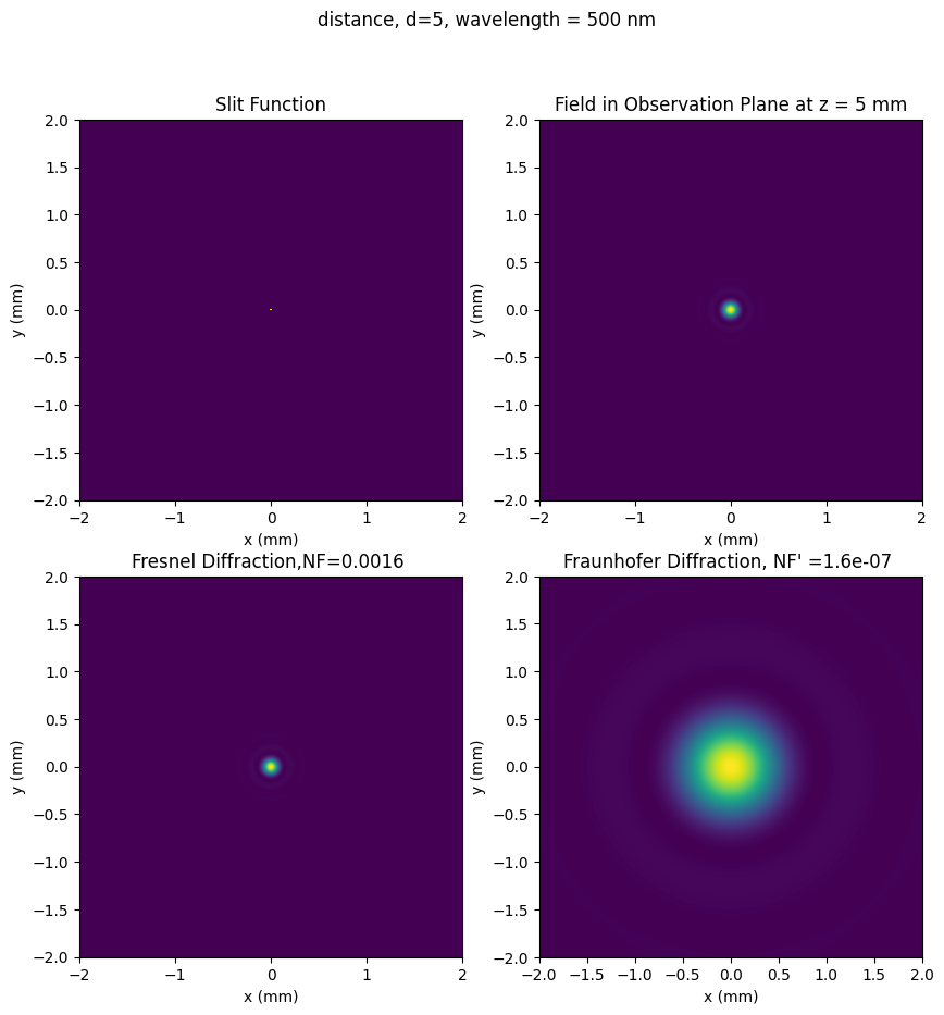
Example 1: Rectangular single slit
# Example-1: Rectangular slit
plt.figure(figsize=(10, 10))    # plot function

wavelength = 500        # Wavelength in nm
D=0.05                   # Slit width in mm, or slit diameter for circular slits
S=0.01                    # Slit separation in mm, only used for double slits
Height =2                # Height of the slit in mm, only used for rectangular slits
d=10                      # Distance from the slit to the observation plane in mm
a=2                      # Size of the observation plane in mm
# Calculate the transfer function for the exact method
method = 'exact'            # Change to 'exact' or 'Fraunhofer' as needed
slit_type = 'rectangular'   # Change to 'circular' or 'double' as needed
x,y,U0,U_exact=transfer_function(method, slit_type, d, wavelength,D,S,Height)


plt.suptitle('distance, d={}, wavelength = {} nm'.format(d,wavelength))
# Plot the slit function
plt.subplot(2, 2, 1)
plt.pcolormesh(x,y,U0)
plt.title('Slit Function')
plt.xlabel('x (mm)')
plt.ylabel('y (mm)')

# Plot the exact diffraction pattern
plt.subplot(2, 2, 2)
plt.title('Field in Observation Plane at z = {} mm'.format(d))
plt.pcolormesh(x,y,np.abs(U_exact)**2)
plt.xlabel('x (mm)')
plt.ylabel('y (mm)')


# Calculate the transfer function for the Fresnel method
Nf=(a**2)/(wavelength*d)        # Fresnel number
method = 'Fresnel'            # Change to 'exact' or 'Fraunhofer' as needed
x,y,U0,U_fresnel=transfer_function(method, slit_type, d, wavelength,D,S,Height)
plt.subplot(2, 2, 3)
plt.pcolormesh(x,y,np.abs(U_fresnel)**2)
plt.title('Fresnel Diffraction,NF={} '.format(Nf))
plt.xlabel('x (mm)')
plt.ylabel('y (mm)')


# Calculate the transfer function for the Fraunhofer method
N_fraunhofer=(Height**2)/(wavelength*d)  # Fraunhofer number
method = 'Fraunhofer'         # Change to 'exact' or 'Fresnel' as needed
x1,y1,U0,U_fraunhofer=transfer_function(method, slit_type, d, wavelength,D,S,Height)
plt.subplot(2, 2, 4)
plt.pcolormesh(x1,y1,np.abs(U_fraunhofer)**2)
plt.title('Fraunhofer Diffraction, NF\' ={} '.format(N_fraunhofer))
plt.xlim(-2,2)
plt.ylim(-1,1)
plt.xlabel('x (mm)')
plt.ylabel('y (mm)')
plt.show()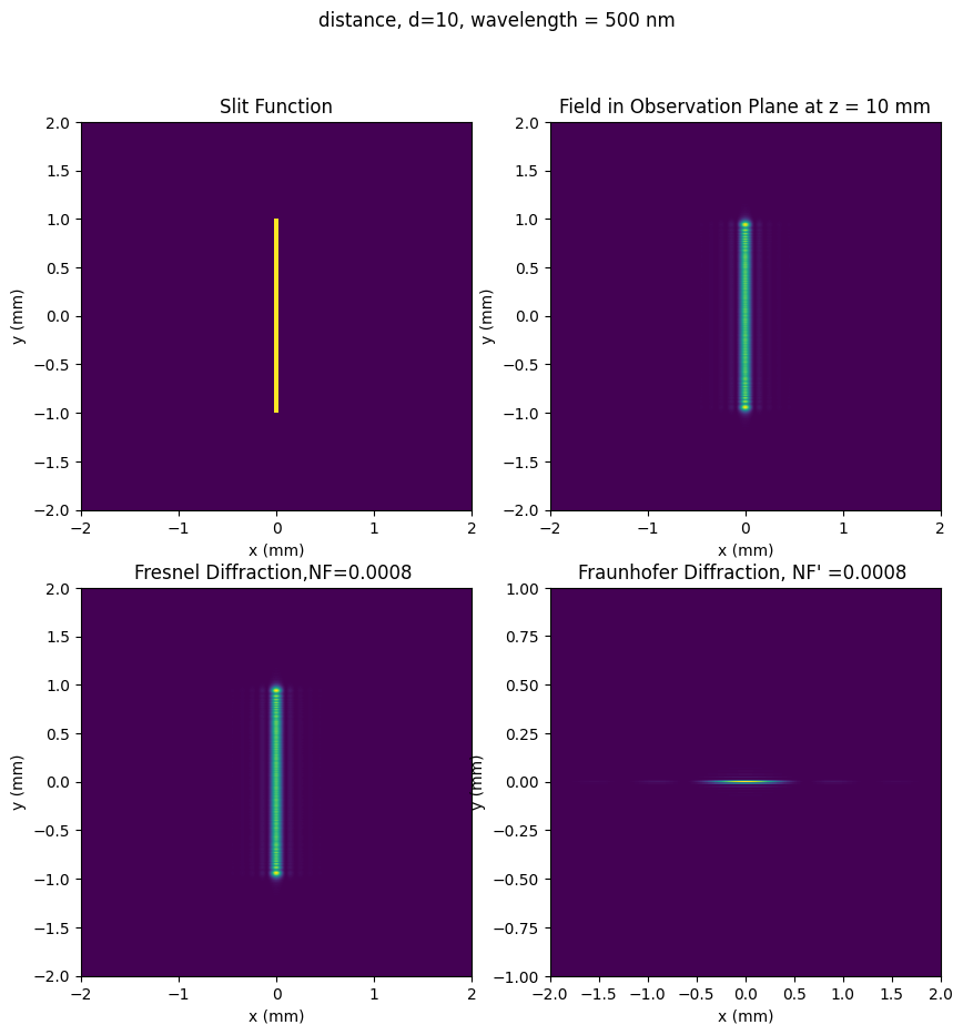
# Plotting the intensity profile along the x-axis at y=0
I_zero=np.abs(U_exact)[250]
plt.plot(x, I_zero)
plt.xlabel('$x$ [mm]')
plt.ylabel('$u(x,y,z)$ [sqrt of intensity]')
plt.xlim([-1,1])
plt.grid()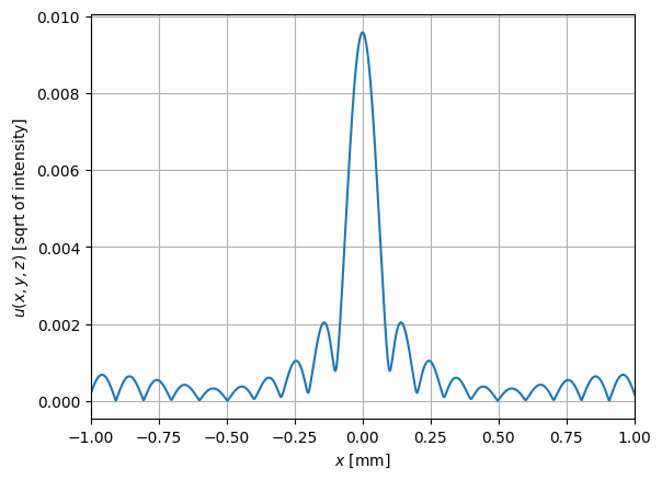
Example 2: Rectangular double slit
# Example-2: Rectangular double slit
plt.figure(figsize=(10, 10))    # plot function

wavelength = 500        # Wavelength in nm
D=0.02                   # Slit width in mm, or slit diameter for circular slits
S=1                    # Slit separation in mm, only used for double slits
Height =2                # Height of the slit in mm, only used for rectangular slits
d=10                      # Distance from the slit to the observation plane in mm
a=2                      # Size of the observation plane in mm
# Calculate the transfer function for the exact method
method = 'exact'            # Change to 'exact' or 'Fraunhofer' as needed
slit_type = 'double'   # Change to 'circular' or 'rectangular' as needed
x,y,U0,U_exact=transfer_function(method, slit_type, d, wavelength,D,S,Height)


plt.suptitle('distance, d={}, wavelength = {} nm'.format(d,wavelength))
# Plot the slit function
plt.subplot(2, 2, 1)
plt.pcolormesh(x,y,U0)
plt.title('Slit Function')
plt.xlabel('x (mm)')
plt.ylabel('y (mm)')

# Plot the exact diffraction pattern
plt.subplot(2, 2, 2)
plt.title('Field in Observation Plane at z = {} mm'.format(d))
plt.pcolormesh(x,y,np.abs(U_exact)**2)
plt.xlabel('x (mm)')
plt.ylabel('y (mm)')


# Calculate the transfer function for the Fresnel method
Nf=(a**2)/(wavelength*d)        # Fresnel number
method = 'Fresnel'            # Change to 'exact' or 'Fraunhofer' as needed
x,y,U0,U_fresnel=transfer_function(method, slit_type, d, wavelength,D,S,Height)
plt.subplot(2, 2, 3)
plt.pcolormesh(x,y,np.abs(U_fresnel)**2)
plt.title('Fresnel Diffraction,NF={} '.format(Nf))
plt.xlabel('x (mm)')
plt.ylabel('y (mm)')


# Calculate the transfer function for the Fraunhofer method
N_fraunhofer=(Height**2)/(wavelength*d)  # Fraunhofer number
method = 'Fraunhofer'         # Change to 'exact' or 'Fresnel' as needed
x1,y1,U0,U_fraunhofer=transfer_function(method, slit_type, d, wavelength,D,S,Height)
plt.subplot(2, 2, 4)
plt.pcolormesh(x1,y1,np.abs(U_fraunhofer)**2)
plt.title('Fraunhofer Diffraction, NF\' ={} '.format(N_fraunhofer))
plt.xlim(-2,2)
plt.ylim(-1,1)
plt.xlabel('x (mm)')
plt.ylabel('y (mm)')
plt.show()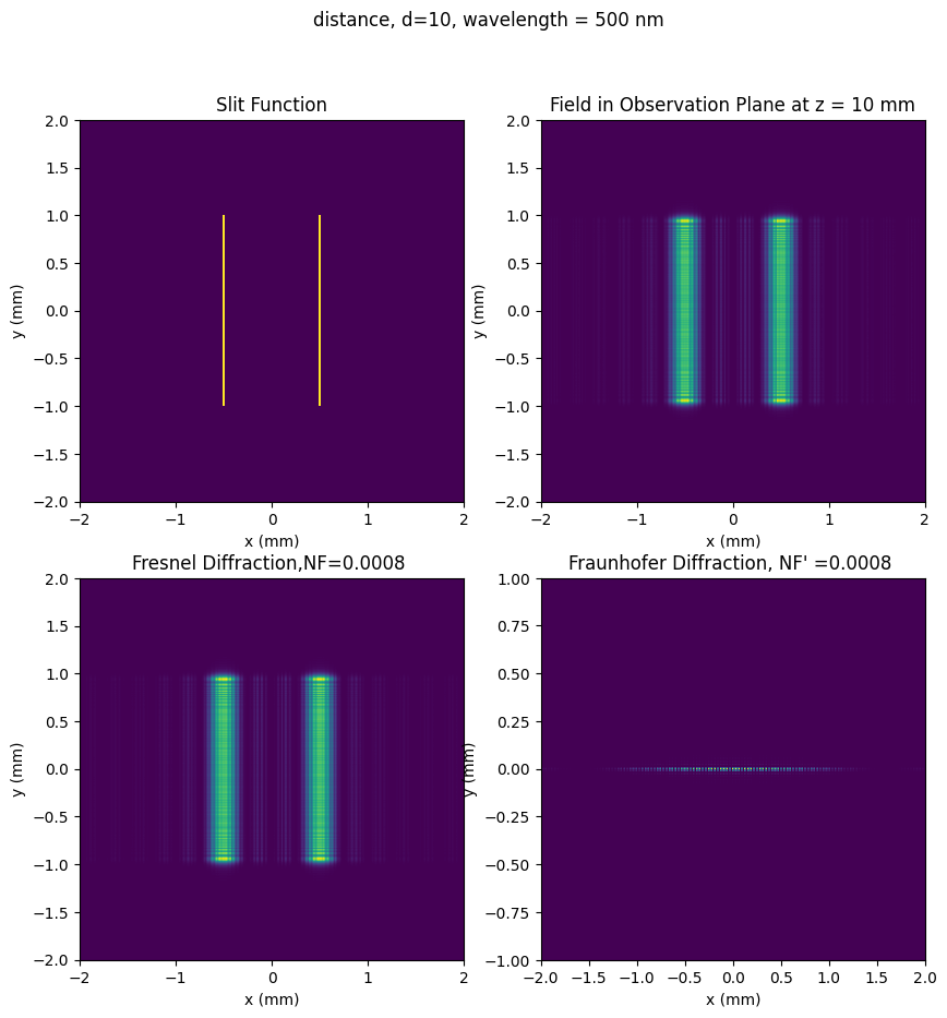
# Plotting the intensity profile along the x-axis at y=0
I_zero=np.abs(U_exact)[250]
plt.plot(x, I_zero)
plt.xlabel('$x$ [mm]')
plt.ylabel('$u(x,y,z)$ [sqrt of intensity]')
plt.xlim([-1,1])
plt.grid()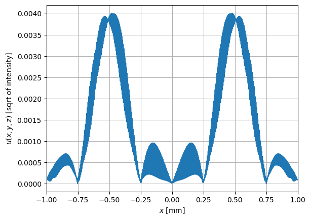
Example 3: Circular slit
# Example-2: Circular slit
plt.figure(figsize=(10, 10))    # plot function

wavelength = 500        # Wavelength in nm
D=0.02                   # Slit width in mm, or slit diameter for circular slits
S=1                    # Slit separation in mm, only used for double slits
Height =2                # Height of the slit in mm, only used for rectangular slits
d=5                      # Distance from the slit to the observation plane in mm
a=2                      # Size of the observation plane in mm
# Calculate the transfer function for the exact method
method = 'exact'            # Change to 'exact' or 'Fraunhofer' as needed
slit_type = 'circular'   # Change to 'circular' or 'rectangular' as needed
x,y,U0,U_exact=transfer_function(method, slit_type, d, wavelength,D,S,Height)


plt.suptitle('distance, d={}, wavelength = {} nm'.format(d,wavelength))
# Plot the slit function
plt.subplot(2, 2, 1)
plt.pcolormesh(x,y,U0)
plt.title('Slit Function')
plt.xlabel('x (mm)')
plt.ylabel('y (mm)')

# Plot the exact diffraction pattern
plt.subplot(2, 2, 2)
plt.title('Field in Observation Plane at z = {} mm'.format(d))
plt.pcolormesh(x,y,np.abs(U_exact)**2)
plt.xlabel('x (mm)')
plt.ylabel('y (mm)')


# Calculate the transfer function for the Fresnel method
Nf=(a**2)/(wavelength*d)        # Fresnel number
method = 'Fresnel'            # Change to 'exact' or 'Fraunhofer' as needed
x,y,U0,U_fresnel=transfer_function(method, slit_type, d, wavelength,D,S,Height)
plt.subplot(2, 2, 3)
plt.pcolormesh(x,y,np.abs(U_fresnel)**2)
plt.title('Fresnel Diffraction,NF={} '.format(Nf))
plt.xlabel('x (mm)')
plt.ylabel('y (mm)')


# Calculate the transfer function for the Fraunhofer method
N_fraunhofer=(D**2)/(wavelength*d)  # Fraunhofer number
method = 'Fraunhofer'         # Change to 'exact' or 'Fresnel' as needed
x1,y1,U0,U_fraunhofer=transfer_function(method, slit_type, d, wavelength,D,S,Height)
plt.subplot(2, 2, 4)
plt.pcolormesh(x1,y1,np.abs(U_fraunhofer)**2)
plt.title('Fraunhofer Diffraction, NF\' ={} '.format(N_fraunhofer))
plt.xlim(-2,2)
plt.ylim(-2,2)
plt.xlabel('x (mm)')
plt.ylabel('y (mm)')
plt.show()